Note
Go to the end to download the full example code.
Kinase affinity due to PTM flanking sequence alterations#
Kinases are known to recognize specific motifs surrounding Y, S, and T residues, and these motifs can be used to predict kinase interactions using a tool called Kinase Library. Here, we will use Kinase Library to identify kinases who may have a stronger preference for the flanking sequences of PTMs in one isoform vs. another. For this example, let’s focus on phosphorylation sites that have larger changes >0.4 in the splicing data.
Note
The optional dependency kinase-library is required to run this example. You can install it using pip install kinase-library.
from ptm_pose import helpers
from ptm_pose.analyze import enzyme

altered_flanks = helpers.load_example_data(altered_flanks=True)

# initialize the kinase library class
klibrary = enzyme.KL_flank_analysis(altered_flanks, min_dpsi = 0.4)
89 PTMs removed due to insignificant splice event (p < 0.05, dpsi >= 0.4): (86.41%)
Final number of PTMs to be assessed: 14
Now that we have the class initialized, we have two options. If there is a specific PTM of interest, we can run the analysis on that specific PTM. Otherwise, we can run the analysis on all PTMs in the dataframe. Let’s analyzing across all PTMs first. This will return a dataframe containing scores of each kinase for every event in the altered_flanks dataframe for both the inclusion and exclusion isoforms. In addition, it will calculate the difference and the relative difference (normalized by dPSI) between the two isoforms: :
klibrary.analyze_all_ptms()
Score sequences for inclusion isoforms
Scoring 12 ser_thr substrates
Calculating percentile for 12 ser_thr substrates

  0%|          | 0/311 [00:00<?, ?it/s]
  5%|▍         | 15/311 [00:00<00:02, 142.01it/s]
 10%|▉         | 30/311 [00:00<00:02, 140.24it/s]
 14%|█▍        | 45/311 [00:00<00:01, 133.92it/s]
 19%|█▉        | 59/311 [00:00<00:01, 133.29it/s]
 23%|██▎       | 73/311 [00:00<00:01, 135.06it/s]
 28%|██▊       | 87/311 [00:00<00:01, 133.73it/s]
 32%|███▏      | 101/311 [00:00<00:01, 133.93it/s]
 38%|███▊      | 117/311 [00:00<00:01, 139.36it/s]
 42%|████▏     | 131/311 [00:00<00:01, 132.01it/s]
 47%|████▋     | 146/311 [00:01<00:01, 134.46it/s]
 52%|█████▏    | 161/311 [00:01<00:01, 138.24it/s]
 56%|█████▋    | 175/311 [00:01<00:00, 136.76it/s]
 61%|██████    | 189/311 [00:01<00:00, 133.89it/s]
 65%|██████▌   | 203/311 [00:01<00:00, 135.16it/s]
 70%|██████▉   | 217/311 [00:01<00:00, 134.35it/s]
 74%|███████▍  | 231/311 [00:01<00:00, 134.96it/s]
 79%|███████▉  | 245/311 [00:01<00:00, 136.32it/s]
 83%|████████▎ | 259/311 [00:01<00:00, 136.70it/s]
 88%|████████▊ | 274/311 [00:02<00:00, 140.46it/s]
 93%|█████████▎| 289/311 [00:02<00:00, 137.88it/s]
 97%|█████████▋| 303/311 [00:02<00:00, 136.45it/s]
100%|██████████| 311/311 [00:02<00:00, 134.62it/s]
Scoring 1 tyrosine substrates
Calculating percentile for 1 tyrosine substrates

  0%|          | 0/78 [00:00<?, ?it/s]
100%|██████████| 78/78 [00:00<00:00, 2571.41it/s]

Scoring sequences for exclusion isoforms
Scoring 12 ser_thr substrates
Calculating percentile for 12 ser_thr substrates

  0%|          | 0/311 [00:00<?, ?it/s]
  5%|▍         | 14/311 [00:00<00:02, 136.40it/s]
  9%|▉         | 28/311 [00:00<00:02, 122.13it/s]
 14%|█▎        | 42/311 [00:00<00:02, 127.18it/s]
 18%|█▊        | 55/311 [00:00<00:02, 118.31it/s]
 22%|██▏       | 67/311 [00:00<00:02, 117.39it/s]
 25%|██▌       | 79/311 [00:00<00:02, 115.36it/s]
 29%|██▉       | 91/311 [00:00<00:01, 116.23it/s]
 33%|███▎      | 104/311 [00:00<00:01, 119.67it/s]
 37%|███▋      | 116/311 [00:00<00:01, 118.90it/s]
 41%|████▏     | 129/311 [00:01<00:01, 121.07it/s]
 46%|████▌     | 142/311 [00:01<00:01, 117.83it/s]
 50%|████▉     | 155/311 [00:01<00:01, 120.13it/s]
 54%|█████▍    | 168/311 [00:01<00:01, 120.57it/s]
 58%|█████▊    | 181/311 [00:01<00:01, 120.87it/s]
 63%|██████▎   | 195/311 [00:01<00:00, 124.19it/s]
 67%|██████▋   | 208/311 [00:01<00:00, 124.03it/s]
 71%|███████   | 221/311 [00:01<00:00, 125.14it/s]
 75%|███████▌  | 234/311 [00:01<00:00, 124.30it/s]
 80%|███████▉  | 248/311 [00:02<00:00, 126.12it/s]
 84%|████████▍ | 261/311 [00:02<00:00, 125.10it/s]
 88%|████████▊ | 274/311 [00:02<00:00, 121.79it/s]
 92%|█████████▏| 287/311 [00:02<00:00, 122.43it/s]
 96%|█████████▋| 300/311 [00:02<00:00, 124.31it/s]
100%|██████████| 311/311 [00:02<00:00, 121.35it/s]
Scoring 1 tyrosine substrates
Calculating percentile for 1 tyrosine substrates

  0%|          | 0/78 [00:00<?, ?it/s]
100%|██████████| 78/78 [00:00<00:00, 2443.92it/s]
With all the scores calculated, we can then identify the sites and events with the largest changes in affinity. To better represent how big of a change this can be, we can calculate a relative affinity change, which is the difference in percentile score change between inclusion and exclusion isoforms, normalized by the change in dPSI. This will give us a better idea of how much the affinity is changing relative to the change in splicing. We can then plot this data to visualize the results.
klibrary.plot_top_changes()
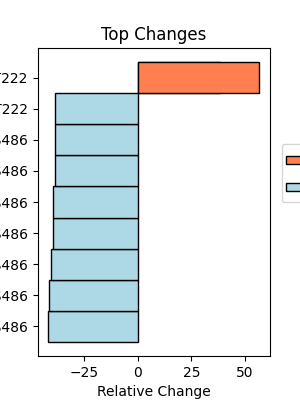
Here, we can see that a site in CD44 has a shift towards interactions with CAMK2G upon the provided perturbation, and our US01 site has several different kinases which prefer the isoform expressed prior to perturbation. In addition to looking at individual sites, we can also see if there are any kinases with consistently large differences in scores/percentiles across the flanking sequence changes. This can be done using the plot_top_kinases() function, which will plot the top kinases with the largest differences in scores across all PTMs (based on median by default). This can be useful for identifying kinases that may be more broadly impacted by the splicing events.
klibrary.plot_top_kinases(top_n = 5)
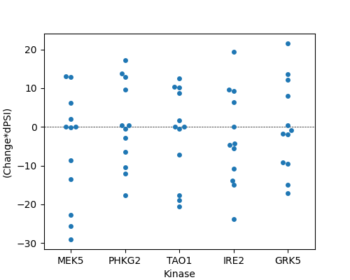
Shown are the top 5 kinases with the largest median difference across all assessed PTMs. You’ll see that many of the PTMs don’t result in a large change, but some kinases, like MEK5, have a large change in preference after perturbation for some sites.
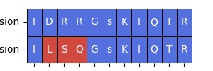
Now let’s say we didn’t want to focus on a specific PTM, such as the USO1 S486 site. We can do this by using the analyze_single_ptm() function, which will return a dataframe with the scores of each kinase for the inclusion and exclusion isoforms, as well as the difference and relative difference between the two isoforms for the specified PTM. First, let’s take a look at what the flanking sequences look like for this PTM:
gene = 'USO1'
loc = 486
example = altered_flanks[(altered_flanks['Gene'] == gene) & (altered_flanks['PTM Position in Isoform'] == loc)].squeeze()

from ptm_pose.analyze import flank_analysis

flank_analysis.plot_sequence_differences(example['Inclusion Flanking Sequence'], example['Exclusion Flanking Sequence'])
Now we can run the kinase library analysis on this specific PTM. This will return a dataframe with the kinases that have a higher affinity for the inclusion or exclusion isoform, as well as the p-value and fold change.
affinity_change = klibrary.analyze_single_ptm('ARHGAP17', 497)
print(affinity_change.head(10))
       Inclusion percentile  Exclusion percentile  Difference  Absolute Difference   dPSI  Relative Change in Preference
CDK3                   5.57                 93.56      -87.99                87.99  0.413                      -36.33987
CDK1                   7.36                 92.91      -85.55                85.55  0.413                      -35.33215
DRAK1                 97.87                 17.28       80.59                80.59  0.413                       33.28367
CDK2                  18.64                 95.50      -76.86                76.86  0.413                      -31.74318
CLK2                  17.91                 91.13      -73.22                73.22  0.413                      -30.23986
YANK3                 75.92                  3.12       72.80                72.80  0.413                       30.06640
RIPK2                 90.77                 18.16       72.61                72.61  0.413                       29.98793
RIPK3                 79.13                  6.87       72.26                72.26  0.413                       29.84338
PLK4                  77.15                  5.07       72.08                72.08  0.413                       29.76904
TTBK1                 71.18                  1.17       70.01                70.01  0.413                       28.91413
From this analysis, we can start to identify events that might rewire kinase interactions. When paired with analysis of differentially included PTMs, we can start to identify kinases that are more or less likely to be influenced by changes to splicing patterns.
Total running time of the script: (0 minutes 10.063 seconds)